Your gRPC Service as a SQL Table: Building an Interoperable Trino Connector

Bridging the gap between your data warehouse and live production services

Jul 08, 2026

Written by Sarp Kaya, a member of our security platform team who led the development of the gRPC Trino Connector.

Data warehouses are great at storing history. They accumulate events, snapshots, and aggregations over time, and they let you query all of it with SQL. They typically don’t allow you to talk to live services: the ones running in production right now, holding data that never quite belongs in the warehouse.

At Atoms, we see this cause concrete problems: our warehouse held lookup keys for certain fields that lived in an external service. Analysts needed to resolve those keys to actual values, but there was no SQL-native way to do it. Every tool in our stack, including Superset, Jupyter Notebooks, ETL pipelines, and ad-hoc queries, ran through Trino, and none of them could bridge that gap.

The solution we landed on was a gRPC-backed Trino connector: a custom plugin that speaks your service’s protocol directly from the query engine, resolves a batch of keys in a single call, and returns the results as a regular SQL result set. We’ve found the usefulness outweighs the risk to services in many situations.

This post covers how it works, why we designed it the way we did, and a full implementation walkthrough at the end.

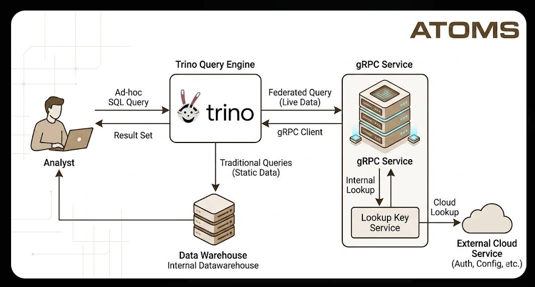
The Core Idea: Services as Tables

Most data in a warehouse gets there via ETL or ELT. A pipeline reads from a source system and writes the data into the warehouse. It’s reliable, it scales well, and it’s the right model for most data. But there are cases where pulling data into the warehouse ahead of time is the wrong approach.

Services Enforcing Access Control:

Authorization logic that goes beyond what a warehouse can model with row-level permissions or table grants. The service decides who sees what based on request context, caller identity, or business rules. Replicating the data into the warehouse means bypassing that entirely.

Ownership:

Once data is copied into the warehouse, the genie is out of the bottle. Anyone with warehouse access has it, and the owning team has lost control over how it’s used, who sees it, and when it gets stale. For data that’s intentionally kept behind a service boundary, replication undermines the whole point.

Freshness:

Some data changes fast enough that ETL snapshots are misleading rather than helpful. The obvious reaction is to skip ETL and connect directly to the service’s database, like a read replica or a Postgres foreign data wrapper. But that only works when the service’s data is a clean set of tables you can query as-is. In practice, many services don’t just store data. They compute it. The value you need might be derived from multiple tables, combined with data from other sources, or produced through business logic that lives in the service code, not in the schema. Connecting to the database directly would mean either replicating that logic in SQL inside the warehouse, which creates a maintenance burden and a source of drift, or accepting that you’re reading raw storage that doesn’t mean what you think it means without the service’s interpretation layer on top.

Financial:

Some data gets queried so infrequently that maintaining a continuous sync pipeline doesn’t make financial sense. A connector lets you pay per query rather than per pipeline run. You only call the service when someone actually needs the data.

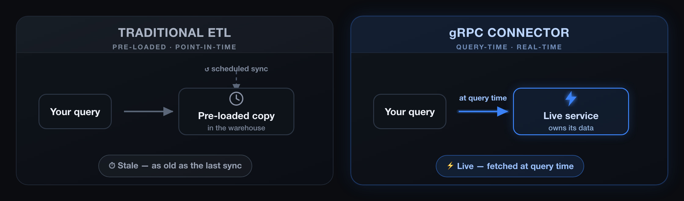
The alternative this connector explores: instead of pulling data into the warehouse ahead of time, let the warehouse call out to the service at query time. The service owns its data, the warehouse issues a real-time request when an analyst needs it, and the response comes back as rows in a SQL result set.

Our Setup: Lookup Keys and an External Service

At Atoms, certain fields are stored in the warehouse as opaque lookup keys, such as strings like k;3f92a104-cd71-4e85-bb3d-72a9f0e8d541. The values live in a dedicated service that exposes a bulk gRPC API: send a list of keys, get back the corresponding values.

-- What the warehouse holds for an externally-owned field:
SELECT lookup_key FROM analytics_views.some_table

-- Result: k;3f92a104-cd71-4e85-bb3d-72a9f0e8d541

Backend services already knew how to call this service over gRPC. The warehouse had no equivalent. Analysts and pipelines were stuck.

The connector closes that gap: it translates a SQL query into a gRPC request, fires it at the service, and returns a result set. From the analyst’s perspective, it’s just another table in Trino.

Why a Connector, Not a UDF?

The first thing most people reach for is a User Defined Function. Trino’s definition of UDF is, a custom function authored by a user of Trino in a client application. UDFs are scalar functions that return a single output value. For more details refer to Trino’s official documentation here.

The problem is that UDFs execute per row. A resolve_key(key) call means a separate gRPC round-trip for every row. For a result set of 500 records, that's 500 sequential calls. At 100ms each, that's 50 seconds just for key resolution.

A connector operates at a different level. Instead of resolving one key at a time, it collects every key from the query, batches them into a single gRPC request, and gets all the results back in one round-trip. The difference is the same query finishing in 100ms instead of 50 seconds.

Trino’s Service Provider Interface (SPI) makes this possible. It lets you build connectors to arbitrary data sources, and a connector that speaks gRPC can participate in query planning, batch keys through dynamic filters, and return results as a standard SQL table. Any future changes to the service’s API are automatically picked up.

Architecture: Trino SPI Meets gRPC

Trino’s SPI requires implementing three interfaces:

ConnectorMetadata describes schemas, tables, and columns to the query planner.
ConnectorSplitManager decides when to execute and packages the work into splits.
ConnectorRecordSetProvider performs the actual data fetch and returns rows to Trino.

The full query lifecycle:

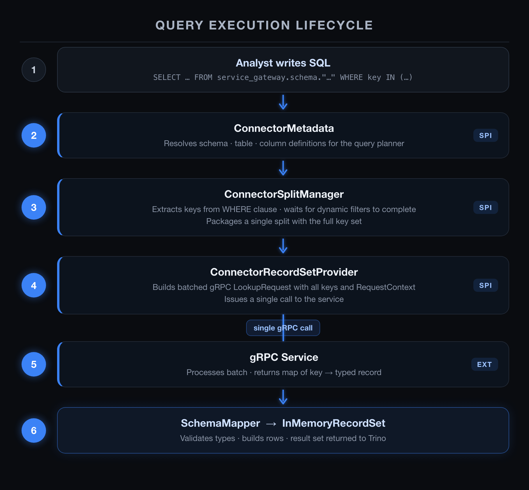
The gRPC client sits inside ConnectorRecordSetProvider. It builds a request proto containing all the lookup keys from the query and fires a single call. The service returns a map of key → value, the mapper converts that to a list of rows, and Trino projects the requested columns.

The connector is registered as a Trino catalog and configured with only two properties: the service host and port. All other details, such as schema definitions, column shapes, and response mapping, are handled within the connector itself.

The gRPC Contract: Request, Response, and Column Mapping

For the connector to work, the gRPC service needs to implement a specific contract. Here’s the shape of that contract:

The request carries a batch of lookup keys and a context block describing who is calling and why. The response maps each key back to a typed result, using a oneof field inside the result message so each data type the service owns gets its own field.

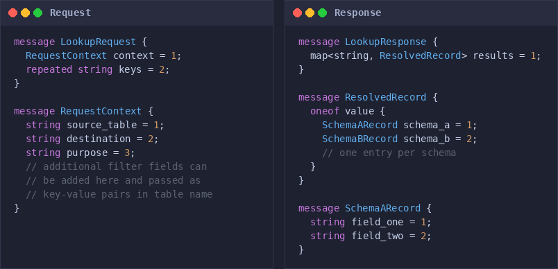
The oneof design keeps the proto schema stable as the service adds new data types. You can simply add a new message and a new field inside the oneof without changing anything else. It also gives the connector a clean way to validate that the response matches what was requested. For example, if you query schema_a but a result comes back with schema_b set, the mapper will drop it.

How the response becomes Trino columns is controlled by a schema mapper. We use one mapper per schema registered in the connector. Each mapper knows which oneof field to read and how to project its proto fields into a Trino row.

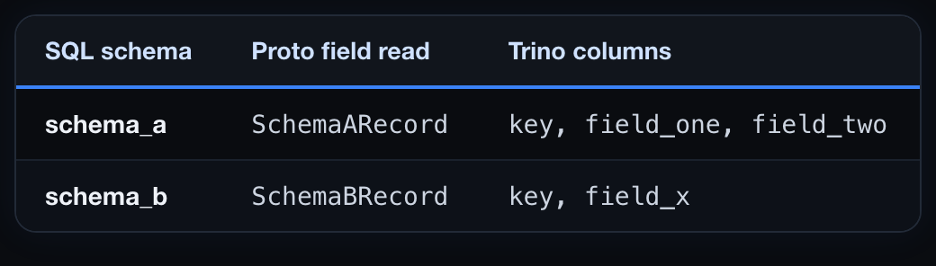
When the connector receives a LookupResponse, it passes each entry to the mapper for the queried schema. The mapper reads the appropriate oneof field, constructs a row, and adds it to the result set. Keys that returned the wrong type or no result at all are silently dropped, so the result set only contains successful resolutions.

Adding a new schema means adding one message to the proto, one field to oneof, one metadata class in the connector (defining the columns), and one mapper class (defining the row construction). The connector’s plumbing doesn’t change.

Request Parameters: How Context Flows from SQL to the Service

Unlike ETL pipelines or direct service calls, SQL queries don’t have a native way to attach per-request metadata. However, the gRPC service needs more than just a list of keys. It needs to know which table the keys came from, what the results will be used for, and the specific data type requested.

These parameters are controlled through three parts of the SQL query itself.

1. The schema name: the specific data type you want.

The schema in the catalog path declares the data type being requested. The connector maps this directly to which oneof field it expects in the response, and which mapper it uses to construct rows.

-- Requesting schema_a records:
FROM service_gateway.schema_a."..."

-- Requesting schema_b records:
FROM service_gateway.schema_b."..."

One query, one schema. Mixing data types in a single query would make response validation significantly harder, so the connector enforces this as a hard constraint.

2. The table name, which carries request context as key-value pairs.

The quoted table name carries the RequestContext fields as a &-delimited string. The connector parses this at query time and populates the RequestContext proto before making the gRPC call:

FROM service_gateway.schema_a."source_table:analytics_views.order_info&destination:reporting_dashboard&purpose:order_summary"

This maps to:

RequestContext {
  source_table: "analytics_views.order_info"
  destination:  "reporting_dashboard"
  purpose:      "order_summary"
}

The fields are defined by the proto contract and validated by the connector before the call is made. An unrecognized key in the table name string causes the query to fail with a parse error rather than silently forwarding garbage context to the service.

3. The WHERE clause, which contains the keys themselves.

The lookup keys are extracted from the WHERE key IN (...) clause. This is the only source of keys for the request, as there is no secondary input channel. The connector collects every key from this clause, including keys resolved through dynamic filters from joins and subqueries, and packages them into the repeated string keys field for a single request.

The WHERE key clause is also mandatory. The connector refuses to execute without one, which prevents full-table scans and ensures every call to the service is explicitly scoped.

Putting it all together: SQL to gRPC, step by step.

SELECT *
FROM service_gateway.schema_a."source_table:analytics_views.order_info&destination:reporting_dashboard&purpose:order_summary"
WHERE key IN ('k;a7d3e891-5c20-4f16-93b8-1d4702cf6a3e', 'k;b812d490-...')

The connector parses the schema, table name, and WHERE clause, builds a gRPC request, and the service returns the resolved values:

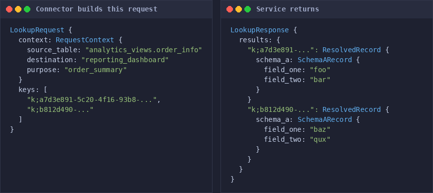
The SchemaAMapper reads each SchemaARecord, maps its fields to the declared Trino columns, and constructs the final result set. That table is what gets returned to Trino, where it can be joined, filtered, or projected like any other SQL result.

Making Joins Work: Dynamic Filters

In practice, analysts pull keys from a warehouse table and join against the connector rather than hardcoding them. Both patterns work:

Subquery:

SELECT *
FROM service_gateway.schema_a."source_table:analytics_views.some_table&destination:reporting_dashboard&purpose:data_enrichment"
WHERE key IN (
    SELECT lookup_key
    FROM analytics_views.some_table
    LIMIT 1000
);

Join:

SELECT t.record_id, t.category, r.field_one, r.field_two
FROM service_gateway.schema_a."source_table:analytics_views.some_table&destination:reporting_dashboard&purpose:data_enrichment" AS r
JOIN (
    SELECT lookup_key, record_id, category
    FROM analytics_views.some_table
    LIMIT 1000
) AS t ON r.key = t.lookup_key;

The mechanism that makes these efficient is Trino’s dynamic filter system. When Trino plans a join, it doesn’t know the full set of join keys yet because the probe side, or the warehouse table, has to execute first. Trino then propagates those key values back to the build side as they are resolved.

The connector’s ServiceGrpcSplitManager participates in this explicitly: it registers a listener on the dynamic filter for the key column and does not produce its split until that filter is complete. Only at that point does it apply the resolved keys to the table handle and package the split.

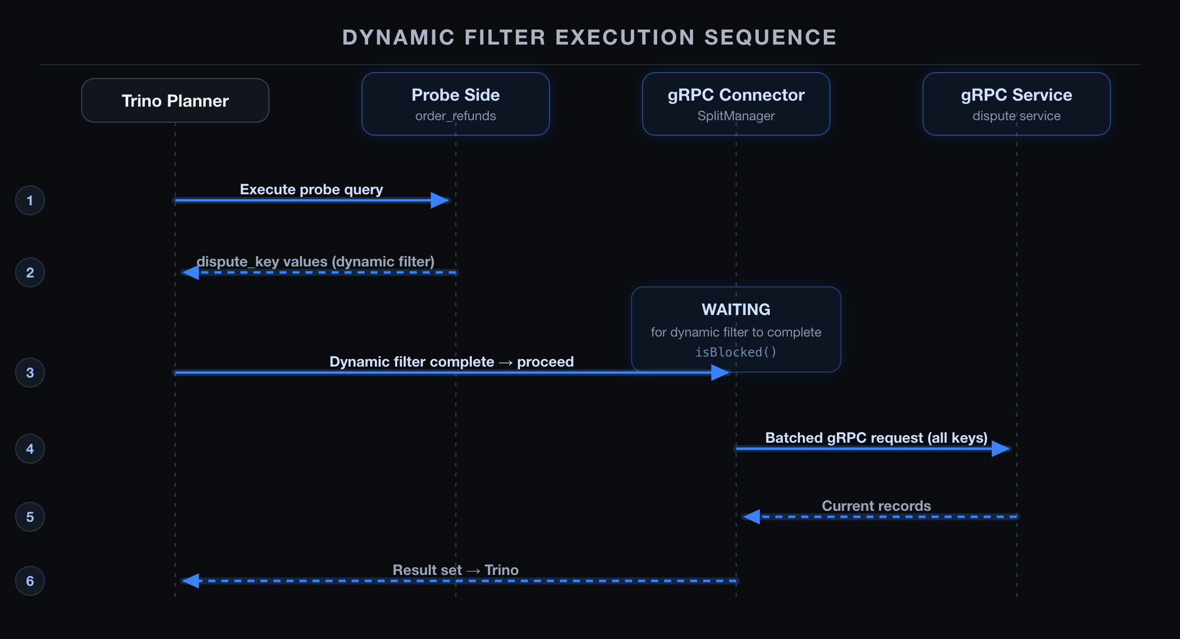
The result: exactly one gRPC call per query, regardless of how many keys are involved. Without dynamic filter participation, you would get one call per row, which is the same problem as the UDF approach, just hidden one layer deeper.

A Concrete Example: Flight Seat Availability

The following is a hypothetical example used purely for illustration. It does not represent any real airline’s architecture or data infrastructure.

To make the above concrete, consider an airline whose data warehouse holds flight schedule and route data: flight numbers, origins, destinations, departure times, aircraft types, and total seat capacity. What the warehouse doesn’t have is live seat availability: how many seats are still open, what the current lowest fare is, and whether a flight is still accepting bookings.

That data lives in a seat inventory service. It’s sensitive and access-controlled: pricing and availability are proprietary, and the service enforces who can query what. It’s also extremely volatile. A flight with 30 open seats at 9 AM might have 4 by noon. ETL snapshots are useless here. You’d be making decisions on stale availability, which in airline revenue management is worse than having no data at all.

With the connector, a revenue analyst can join the warehouse’s schedule data against live seat availability in a single query, and the inventory service stays in full control of access and filtering.

The proto contract for this schema fits into the generic ResolvedRecord shape. The RequestContext gains a booking_status_filter field, which the service uses to filter results server-side before returning them.

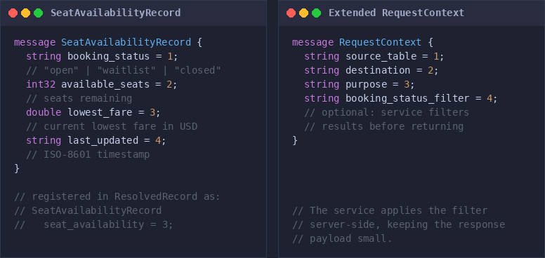
Here’s a query that joins warehouse schedule data against live availability:

SELECT s.flight_number, s.origin, s.destination, s.departure_time, s.aircraft_type,
       a.booking_status, a.available_seats, a.lowest_fare, a.last_updated
FROM service_gateway.seat_availability."source_table:flight_schedule&destination:revenue_mgmt&purpose:availability_overview" AS a
JOIN (
    SELECT flight_id, flight_number, origin, destination, departure_time, aircraft_type
    FROM analytics_views.flight_schedule
    LIMIT 1000
) AS s ON a.key = s.flight_id;

The warehouse contributes the schedule context (flight number, route, aircraft type). The connector contributes the live state (booking status, seats remaining, current fare). The result is a single joined table:

To narrow the results, you add a booking_status_filter to the table name string. For example, booking_status_filter:open tells the service to return only flights still accepting bookings. The same three keys are sent either way, but the service decides what to return based on the filter. The filtering happens server-side, keeping the response payload small and the work where the data lives.

Performance in Production

Measured latency in production:

gRPC service end-to-end: Approximately 75 to 100ms for a full batch.
Trino connector layer: ~100ms total per query
Overhead vs. equivalent queries without service calls: Negligible

A 100ms round-trip is negligible compared to the total execution time of a real analytical query. Analysts don’t notice it. The comparison that really matters isn’t connector versus no connector, but rather how it compares to alternatives that either didn’t exist or couldn’t scale. In that regard, the connector is the clear winner.

Lessons

Speak the same protocol your services already speak. If that’s gRPC, the connector uses it directly. No translation layer, no REST adapter, no schema negotiation. Just a typed protobuf request and response. If your services use something else, the pattern still applies. The connector is the hard part; swapping the transport underneath it is not.

One call per query, not one call per row. The dynamic filter, the mandatory WHERE key clause, and the single-split model all ensure the connector makes one batched call per query. That said, once you give SQL users a live line to a production service, you need to think about protecting that service. Timeouts, rate limiting, adaptive concurrency, caching at both the connector and service layer, tiered SLAs where Trino traffic gets lower priority, dedicated service pods for connector traffic. These are standard distributed systems tools and the right mix depends on your traffic patterns. The connector doesn't prescribe a specific strategy, but it does enforce a key limit per request as a baseline safeguard.

Solve it at the query engine, not at the tools. Implementing this in Trino means every tool that touches the warehouse gets service resolution automatically. Tools like Superset, Jupyter Notebooks, and ETL pipelines don’t need any changes. The connector acts as an infrastructure primitive that works everywhere Trino does.

Put the context in the query, not next to it. We encode call context directly in the table name. It looks weird, but it means the query carries everything the service needs: where the keys came from, what the results are for, which schema to resolve. No session properties to set, no config files to maintain, no metadata store to coordinate with. Superset, Notebooks, ETL pipelines, they all just run SQL. They don't know about the connector and they don't need to.

The oneof response shape pays off over time. Designing the service response as a typed discriminated union keeps validation reliable and ensures the proto contract remains stable as you add new schemas. Every new data type fits into the existing message structure without requiring changes elsewhere.

The broader takeaway is that Trino’s SPI isn’t just for databases. It is an extension point for any service that can handle a batched request. If your team runs gRPC services with data that doesn’t belong in the warehouse, a connector gives SQL users a direct line to it without requiring ETL.

Future Work

Today the connector enforces a hard key limit per request. If the key set exceeds it, the query fails and the analyst has to narrow their selection. This is intentional for now, but limiting. The next step is partitioning large key sets across multiple splits in the SplitManager so Trino can schedule them across workers and merge the results. The harder problem is making sure that doesn’t hammer the service. Queuing splits, controlling concurrency, applying per-split timeouts, and handling partial failures all need to be in place before we remove the key limit safely.

Implementation:

See our implementation guideline here.

Discussion about this post

Ready for more?